Excel text function
TEXT function
The TEXT function lets you change the way a number appears by applying formatting to it with format codes. It’s useful in situations where you want to display numbers in a more readable format, or you want to combine numbers with text or symbols.
Note: The TEXT function will convert numbers to text, which may make it difficult to reference in later calculations. It’s best to keep your original value in one cell, then use the TEXT function in another cell. Then, if you need to build other formulas, always reference the original value and not the TEXT function result.
The TEXT function syntax has the following arguments:
A numeric value that you want to be converted into text.
A text string that defines the formatting that you want to be applied to the supplied value.
Overview
In its simplest form, the TEXT function says:
=TEXT(Value you want to format, «Format code you want to apply»)
Here are some popular examples, which you can copy directly into Excel to experiment with on your own. Notice the format codes within quotation marks.
Currency with a thousands separator and 2 decimals, like $1,234.57. Note that Excel rounds the value to 2 decimal places.
Today’s date in MM/DD/YY format, like 03/14/12
Today’s day of the week, like Monday
Current time, like 1:29 PM
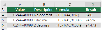
Percentage, like 28.5%
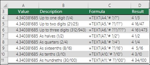
Fraction, like 4 1/3
Fraction, like 1/3. Note this uses the TRIM function to remove the leading space with a decimal value.
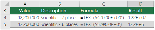
Scientific notation, like 1.22E+07
Add leading zeros (0), like 0001234
Note: Although you can use the TEXT function to change formatting, it’s not the only way. You can change the format without a formula by pressing CTRL+1 (or  +1 on the Mac), then pick the format you want from the Format Cells > Number dialog.
Download our examples
You can download an example workbook with all of the TEXT function examples you’ll find in this article, plus some extras. You can follow along, or create your own TEXT function format codes.
Other format codes that are available
You can use the Format Cells dialog to find the other available format codes:
Press Ctrl+1 ( +1 on the Mac) to bring up the Format Cells dialog.
Select the format you want from the Number tab.
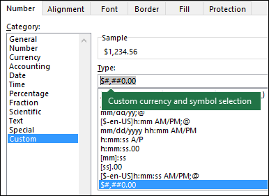
Select the Custom option,
The format code you want is now shown in the Type box. In this case, select everything from the Type box except the semicolon (;) and @ symbol. In the example below, we selected and copied just mm/dd/yy.
Press Ctrl+C to copy the format code, then press Cancel to dismiss the Format Cells dialog.
Now, all you need to do is press Ctrl+V to paste the format code into your TEXT formula, like: =TEXT(B2,» mm/dd/yy«). Make sure that you paste the format code within quotes («format code»), otherwise Excel will throw an error message.
 Cells > Number > Custom dialog to have Excel create format strings for you.» xmlns_AntiXSS=»urn:AntiXSSExtensions» />
Format codes by category
Following are some examples of how you can apply different number formats to your values by using the Format Cells dialog, then use the Custom option to copy those format codes to your TEXT function.
- Select a number format
- Leading zero’s (0’s)
- Display a thousands separator
- Number, currency and accounting formats
- Dates
- Times
- Percentages
- Fractions
- Scientific notation
- Special formats
Why does Excel delete my leading 0’s?
Excel is trained to look for numbers being entered in cells, not numbers that look like text, like part numbers or SKU’s. To retain leading zeros, format the input range as Text before you paste or enter values. Select the column, or range where you’ll be putting the values, then use CTRL+1 to bring up the Format > Cells dialog and on the Number tab select Text. Now Excel will keep your leading 0’s.
If you’ve already entered data and Excel has removed your leading 0’s, you can use the TEXT function to add them back. You can reference the top cell with the values and use =TEXT(value,»00000″), where the number of 0’s in the formula represents the total number of characters you want, then copy and paste to the rest of your range.
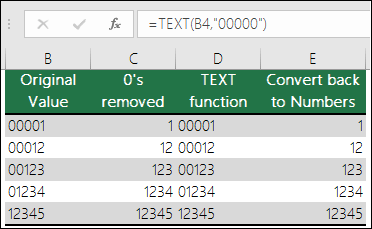
If for some reason you need to convert text values back to numbers you can multiply by 1, like =D4*1, or use the double-unary operator (—), like =—D4.
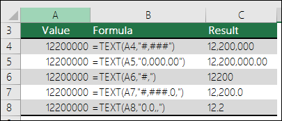
Excel separates thousands by commas if the format contains a comma (,) that is enclosed by number signs (#) or by zeros. For example, if the format string is «#,###», Excel displays the number 12200000 as 12,200,000.
A comma that follows a digit placeholder scales the number by 1,000. For example, if the format string is «#,###.0,», Excel displays the number 12200000 as 12,200.0.
The thousands separator is dependent on your regional settings. In the US it’s a comma, but in other locales it might be a period (.).
The thousands separator is available for the number, currency and accounting formats.
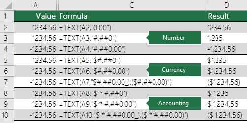
Following are examples of standard number (thousands separator and decimals only), currency and accounting formats. Currency format allows you to insert the currency symbol of your choice and aligns it next to your value, while accounting format will align the currency symbol to the left of the cell and the value to the right. Note the difference between the currency and accounting format codes below, where accounting uses an asterisk (*) to create separation between the symbol and the value.
To find the format code for a currency symbol, first press Ctrl+1 (or +1 on the Mac), select the format you want, then choose a symbol from the Symbol drop-down:
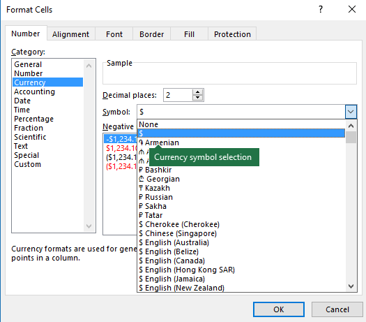
Then click Custom on the left from the Category section, and copy the format code, including the currency symbol.
Note: The TEXT function does not support color formatting, so if you copy a number format code from the Format Cells dialog that includes a color, like this: $#,##0.00_); [Red]($#,##0.00), the TEXT function will accept the format code, but it won’t display the color.
You can alter the way a date displays by using a mix of «M» for month, «D» for days, and «Y» for years.
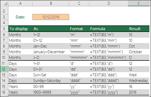
Format codes in the TEXT function aren’t case sensitive, so you can use either «M» or «m», «D» or «d», «Y» or «y».

If you share Excel files and reports with users from different countries, then you might want to give them a report in their language. Excel MVP, Mynda Treacy has a great solution in this Excel Dates Displayed in Different Languages article. It also includes a sample workbook you can download.
You can alter the way time displays by using a mix of «H» for hours, «M» for minutes, or «S» for seconds, and «AM/PM» for a 12-hour clock.
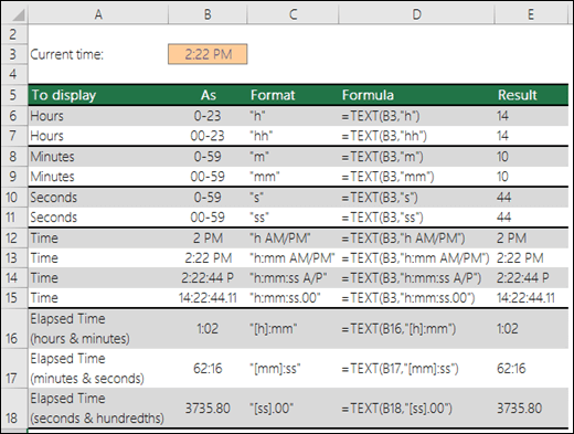
If you leave out the «AM/PM» or «A/P», then time will display based on a 24-hour clock.
Format codes in the TEXT function aren’t case sensitive, so you can use either «H» or «h», «M» or «m», «S» or «s», «AM/PM» or «am/pm».
You can alter the way decimal values display with percentage (%) formats.
You can alter the way decimal values display with fraction (?/?) formats.
Scientific notation is a way of displaying numbers in terms of a decimal between 1 and 10, multiplied by a power of 10. It is often used to shorten the way that large numbers display.
Excel provides 4 special formats:
Zip Code — «00000»
Zip Code + 4 — «00000-0000»
Phone Number — «[ Format Cells > Custom dialog.
Common scenario
The TEXT function is rarely used by itself, and is most often used in conjunction with something else. Let’s say you want to combine text and a number value, like “Report Printed on: 03/14/12”, or “Weekly Revenue: $66,348.72”. You could type that into Excel manually, but that defeats the purpose of having Excel do it for you. Unfortunately, when you combine text and formatted numbers, like dates, times, currency, etc., Excel doesn’t know how you want to display them, so it drops the number formatting. This is where the TEXT function is invaluable, because it allows you to force Excel to format the values the way you want by using a format code, like «MM/DD/YY» for date format.
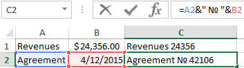
In the following example, you’ll see what happens if you try to join text and a number without using the TEXT function. In this case, we’re using the ampersand ( &) to concatenate a text string, a space (» «), and a value with =A2&» «&B2.
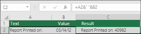
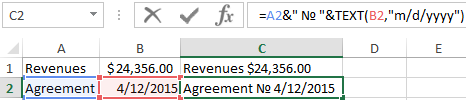
As you can see, Excel removed the formatting from the date in cell B2. In the next example, you’ll see how the TEXT function lets you apply the format you want.
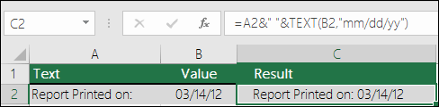
Our updated formula is:
Cell C2: =A2&» «&TEXT(B2,»mm/dd/yy») — Date format
Frequently Asked Questions
Unfortunately, you can’t do that with the TEXT function, you need to use Visual Basic for Applications (VBA) code. The following link has a method: How to convert a numeric value into English words in Excel
Yes, you can use the UPPER, LOWER and PROPER functions. For example, =UPPER(«hello») would return «HELLO».
Yes, but it takes a few steps. First, select the cell or cells where you want this to happen and use Ctrl+1 to bring up the Format > Cells dialog, then Alignment > Text control > check the Wrap Text option. Next, adjust your completed TEXT function to include the ASCII function CHAR(10) where you want the line break. You might need to adjust your column width depending on how the final result aligns.
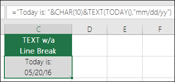
In this case, we used: =»Today is: «&CHAR(10)&TEXT(TODAY(),»mm/dd/yy»)
This is called Scientific Notation, and Excel will automatically convert numbers longer than 12 digits if a cell(s) is formatted as General, and 15 digits if a cell(s) is formatted as a Number. If you need to enter long numeric strings, but don’t want them converted, then format the cells in question as Text before you input or paste your values into Excel.
If you share Excel files and reports with users from different countries, then you might want to give them a report in their language. Excel MVP, Mynda Treacy has a great solution in this Excel Dates Displayed in Different Languages article. It also includes a sample workbook you can download.
The Excel TEXT Function
Function Description
The Excel Text function converts a supplied numeric value into text, in a user-specified format.
The syntax of the function is:
Where the function arguments are:
| value | — | A numeric value, that you want to be converted into text. |
| format_text | — | A text string that defines the formatting that you want to be applied to the supplied value . |
The format definitions that can be used in the Excel Text function are shown in the table below. These definitions have the same meaning when used in the custom style of Excel Cell Formatting.
| 0 | — | Forces the display of a digit in its place |
| # | — | Display digit if it adds to the accuracy of the number (but don’t display if a leading zero or a zero at the end of a decimal) |
| . | — | Defines the position that the decimal place takes |
| d | — | Day of the month or day of week d = one or two digit representation (e.g. 1, 12) dd = 2 digit representation (e.g. 01, 12) ddd = abbreviated day of week (e.g. Mon, Tue) dddd = full name of day of week (e.g. Monday, Tuesday) |
| m | — | Month (when used as part of a date) m = one or two digit representation (e.g. 1, 12) mm = two digit representation (e.g. 01, 12) mmm = abbreviated month name (e.g. Jan, Dec) mmmm = full name of month (e.g. January, December) |
| y | — | Year yy = 2-digit representation of year(e.g. 99, 08) yyyy = 4-digit representation of year(e.g. 1999, 2008) |
| h | — | Hour h = one or two digit representation (e.g. 1, 20) h = two digit representation (e.g. 01, 20) |
| m | — | Minute (when used as a part of a time) m = one or two digit representation (e.g. 1, 55) m = two digit representation (e.g. 01, 55) |
| s | — | Second s = one or two digit representation (e.g. 1, 45) ss = two digit representation (e.g. 01, 45) |
| AM/PM | — | Indicates that a time should be represented using a 12-hour clock, followed by «AM» or «PM» |
Text Function Examples
Example 1
The following spreadsheet shows the Excel Text function, used to apply different formatting types to various numeric values.
| A | B | |
|---|---|---|
| 1 | Value | Formatted Value |
| 2 | 07/07/2015 | =TEXT(A2, «mm/dd/yyyy») |
| 3 | 42192 | =TEXT(A3, «mm/dd/yyyy») |
| 4 | 42192 | =TEXT(A4, «mmm dd yyyy») |
| 5 | 18:00 | =TEXT(A5, «hh:mm») |
| 6 | 0.75 | =TEXT(A6, «hh:mm») |
| 7 | 36.363636 | =TEXT(A7, «0.00») |
| 8 | 0.5555 | =TEXT(A8, «0.0%») |
| 9 | 567.9 | =TEXT(A9, «$#,##0.00») |
| 10 | -5 | =TEXT(A10, «+ $#,##0.00;- $#,##0.00;$0.00») |
| 11 | 5 | =TEXT(A11, «+ $#,##0.00;- $#,##0.00;$0.00») |
| 12 | 0 | =TEXT(A12, «+ $#,##0.00;- $#,##0.00;$0.00») |
| A | B | |
|---|---|---|
| 1 | Value | Formatted Value |
| 2 | 07/07/2015 | 07/07/2015 |
| 3 | 42192 | 07/07/2015 |
| 4 | 42192 | Jul 07 2015 |
| 5 | 18:00 | 18:00 |
| 6 | 0.75 | 18:00 |
| 7 | 36.363636 | 36.36 |
| 8 | 0.5555 | 55.6% |
| 9 | 567.9 | $567.90 |
| 10 | -5 | — $5.00 |
| 11 | 5 | + $5.00 |
| 12 | 0 | $0.00 |
Note that the results returned from the Text function are all text values.
Example 2
One of the most common uses of the Excel Text function is to insert dates into text strings.
Without the use of the Text function, the simple concatenation of a date returns the date’s underlying integer value. This is shown in the example below:
| A | B | C | ||
|---|---|---|---|---|
| 1 | Name | DOB | Name & DOB | |
| 2 | John SMITH | 03/03/1976 | =A2 & » » & B2 | — simple concatenation of date |
| 3 | =A2 & » » & TEXT(B2,»mm/dd/yyyy») | — concatenation using Text function |
| A | B | C | ||
|---|---|---|---|---|
| 1 | Name | DOB | Name & DOB | |
| 2 | John SMITH | 03/03/1976 | John SMITH 27822 | — uses date’s underlying integer value |
| 3 | John SMITH 03/03/1976 | — gives the expected result |
For further details and examples of the Excel Text function, see the Microsoft Office website.
Excel Text Function Common Error
Some users have problems when the Excel Text function returns the #NAME? error:
This is returned from the Excel Text function, if you omit the quotation marks from around the format_text argument.
For example, the formula
will return the #NAME? error.
Solution: Add quotes around the formatting definition.
TEXT Function
What is the Excel TEXT Function?
The Excel TEXT Function is used to convert numbers to text within a spreadsheet. Essentially, the function will convert a numeric value into a text string. TEXT is available in all versions of Excel.
Formula
=Text(Value, format_text)
Value is the numerical value that we need to convert to text
Format_text is the format we want to apply
When is the Excel TEXT Function required?
We use the TEXT function in the following circumstances:
- When we want to display dates in a specified format
- When we wish to display numbers in a specified format or in a more legible way
- When we wish to combine numbers with text or characters
Examples
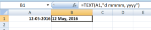
1. Basic example – Excel Text Function
With the following data, I need to convert the data to “d mmmm, yyyy” format. When we insert the text function, the result would look as follows:
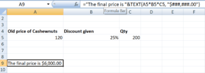
2. Using Excel TEXT with other functions
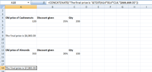
We use the old price and the discount given in cells A5 and B5. The quantity is given in C5. We wish to show some text along with the calculations. We wish to display the information as follows:
The final price is $xxx
Where xxx would be the price in $ terms.
For this, we can use the formula:
=”The final price is “&TEXT(A5*B5*C5, “$###,###.00”)
The other way to do it by using the CONCATENATE function as shown below:
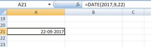
3. Combining the text given with data using TEXT function
When I use the date formula, I would get the result below:
Now, if we try to combine today’s date using CONCATENATE, Excel would give a weird result as shown below:
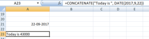
What happened here was that dates that are stored as numbers by Excel were returned as numbers when the CONCATENATE function is used.
To fix it, we need to use the Excel TEXT function. The formula to be used would be:
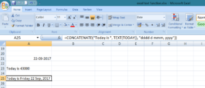
4. Adding zeros before numbers with variable lengths
We all know any zero’s added before numbers are automatically removed by Excel. However, if we need to keep those zeros then the TEXT function comes handy. Let’s see an example to understand how to use this function.
We are given a 9-digit product code, but Excel removed the zeros before it. We can use TEXT as shown below and convert the product code into a 9-digit number:
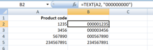
In the above formula, we are given the format code containing 9-digit zeros, where the number of zeros is equal to the number of digits we wish to display.
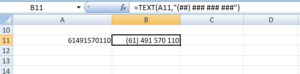
5. Converting telephone numbers to a specific format
If we wish to do the same for telephone numbers, it would involve the use of dashes and parentheses in format codes.
Here, I want to ensure the country code comes in brackets (). Hence the formula used is (##) ### ### ###. The # is the number of digits we wish to use.
To learn more, launch our free Excel crash course now!
Format Code
It is quite easy to use TEXT Function in Excel but it works only when the correct format code is provided. Some frequently used format codes include:
| Code | Description | Example |
|---|---|---|
| # (hash) | It does not display extra zeros | #.# displays a single decimal point. If we input 5.618, it will display 5.6. |
| 0 (zero) | It displays insignificant zeros | #.000 would always display 3 decimals after the number. So if we input 5.68, it will display 5.680. |
| , (comma) | It is a thousand separator | ###,### would put a thousands separator. So if we input 259890, it will display 259,890. |
If the Excel TEXT function isn’t working
Sometimes, the TEXT function will give an error “#NAME?”. This happens when we skip the quotation marks around the format code.
Let’s take an example to understand this.
If we input the formula =TEXT(A2, mm-dd-yy). It would give an error because the formula is incorrect and should be written this way: =TEXT(A2,”mm-dd-yy”).
- The data converted into text cannot be used for calculations. If needed, we should keep the original data in a hidden format and use it for other formulas.
- The characters that can be included in the format code are:
| + | Plus sign |
| — | Minus sign |
| () | Parenthesis |
| : | Colon |
| <> | Curly brackets |
| = | Equal sign |
| Tilde | |
| / | Forward slash |
| ! | Exclamation mark |
| <> | Less than and greater than |
- TEXT function is language-specific. It requires the use of region-specific date and time format codes.
Free Excel Course
Check out our Free Excel Crash Course and work your way toward becoming an expert financial analyst. Learn how to use Excel functions and create sophisticated financial analysis and financial modeling.
Additional Resources
Thanks for reading CFI’s guide to important Excel functions! By taking the time to learn and master these functions, you’ll significantly speed up your financial analysis. To learn more, check out these additional CFI resources:
- Excel Functions for Finance Excel for Finance This Excel for Finance guide will teach the top 10 formulas and functions you must know to be a great financial analyst in Excel. This guide has examples, screenshots and step by step instructions. In the end, download the free Excel template that includes all the finance functions covered in the tutorial
- Advanced Excel Formulas Course
- Advanced Excel Formulas You Must Know Advanced Excel Formulas Must Know These advanced Excel formulas are critical to know and will take your financial analysis skills to the next level. Advanced Excel functions you must know. Learn the top 10 Excel formulas every world-class financial analyst uses on a regular basis. These skills will improve your spreadsheet work in any career
- Excel Shortcuts for PC and Mac Excel Shortcuts PC Mac Excel Shortcuts — List of the most important & common MS Excel shortcuts for PC & Mac users, finance, accounting professions. Keyboard shortcuts speed up your modeling skills and save time. Learn editing, formatting, navigation, ribbon, paste special, data manipulation, formula and cell editing, and other shortucts
Functions for working with text in Excel
For the convenience of working with text in Excel, there are text functions. They make it easy to process hundreds of lines at once. Let’s consider some of them on examples.
Examples with TEXT function in Excel
This function converts numbers to string in Excel. Syntax: value (numeric or reference to a cell with a formula that gives a number as a result); Format (to display the number in the form of text).
The most useful feature of the TEXT function is the formatting of numeric data for merging with text data. Excel «doesn’t understand» how to display numbers without using the function. The program just converts them to a basic format.
Let’s see an example. Let’s say you need to combine text in string with numeric values:
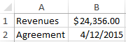
Using an ampersand without a function TEXT produces an inadequate result:
Excel returned the sequence number for the date and the general format instead of the monetary. The TEXT function is used to avoid this. It formats the values according to the user’s request.
The formula «for a date» now looks like this:
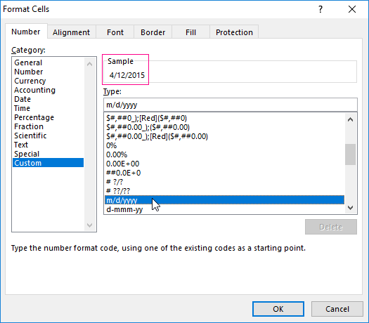
The second argument to the function is the format. Where to take the format line? Right-click on the cell with the value. Click on «Format Cells». In the opened window select «Custom». Copy the required «Type:» in the line. We paste the copied value in the formula.
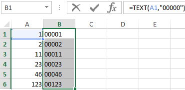
Let’s consider another example where this function can be useful. Add zeros at the beginning of the number. Excel will delete them if you enter it manually. Therefore, we introduce the formula:
If you want to return the old numeric values (without zeros), then use the «—» operator:
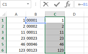
Note that the values are now displayed in numerical format.
Text splitting function in Excel
Individual functions and their combinations allow you to distribute words from one cell to separate cells:
- LEFT (Text, number of characters) displays the specified number of characters from the beginning of the cell;
- RIGHT (Text, number of characters) returns a specified number of characters from the end of the cell;
- SEARCH (Search text, range to search, start position) shows the position of the first occurrence of the searched character or line while viewing from left to right.
The line takes into account the position of each character when dividing the text. Spaces show the beginning or the end of the name you are looking for.
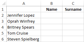
We will split the name, surname and patronymic name into different columns using the functions.
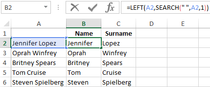
The first line contains only the first and last names separated by a space. Formula for retrieving the name:
The function SEARCH is used to determine the second argument of the LEFT function (the number of characters). It finds a space in cell A2 starting from the left.
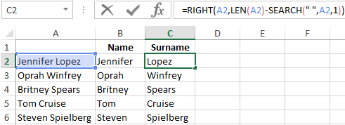
For a name, we use the same formula:
Excel determines the number of characters for the RIGHT function using the SEARCH function. The LEN function «counts» the total length of the text. Then the number of characters up to the first space (found by SEARCH) is subtracted.
The formula for extracting the surname:
Next formulas for extracting the surname is a bit different:
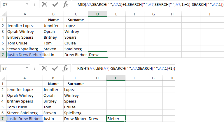
These are five signs on the right. Embedded SEARCH functions search for the second and third spaces in a string. SEARCH («»;A7;1) finds the first space on the left (before the patronymic name). Add one (+1) to the result. We get the position with which we will search for the second space.
Part of the formula SEARCH(» «;A7;SEARCH(» «;A7;1)+1) finds the second space. This will be the final position of the patronymic.
Then the number of characters from the beginning of the line to the second space is subtracted from the total length of the line. The result is the number of characters to the right that you need to return.
Function for merging text in Excel
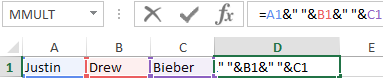
Use the ampersand (&) operator or the CONCATENATE function to combine values from several cells into one line.
For example, the values are located in different columns (cells):
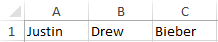
Put the cursor in the cell where the combined three values will be. Enter «=». Select the first cell and click on the keyboard «&» sign. Then enter the space character enclosed in quotation marks (» «). Enter again «&». Therefore, sequentially connect cells with symbols and spaces.
We get the combined values in one cell:
Using the CONCATENATE function:
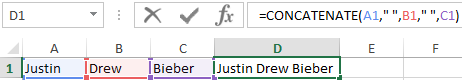
You can add any sign or string to the final expression using quotation marks in the formula.
Text SEARCH function in Excel
The SEARCH function returns the starting position of the searched text (not case sensitive). For example:
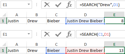
The SEARCH returned to position 8 because the word «Drew» begins with the tenth character in the line. Where can this be useful?
The SEARCH function determines the position of the character in the string line. And the MID function returns symbols values (see the example above). Alternatively, you can replace the found text with the REPLACE.
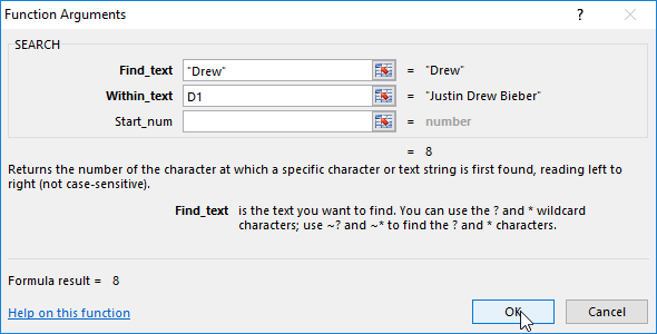
The syntax of the SEARCH function:
- «Find_text» is what you need to find;
- «Withing_text» is where to look;
- «Start_num» is from which position to start searching (by default it is 1).
Use the FIND if you need to take into account the case (lower and upper).